Crash-Course: The Hello World of Machine Learning, Regression

Mikhail Nilov on Pexels

Linear regression is the oldest and most renowned machine learning algorithm out there. It’s the first thing anyone learns about when they start their Machine Learning journey. That is why you could say Linear regression is the “Hello World” of machine learning; all machine learning engineers should know it inside out.

That’s what I’m going to do in this article — teach you everything about linear regression, starting from its history.

One algorithm to start them all

Linear regression is as old as it gets. It was first used under the name of “method of least squares” in 1805, by Adrien-Marie Legendre. Carl Friedrich Gauss allegedly claimed that he used Regression long before anyone else did, and thought it was a trivial technique that anyone would know how to use. The truth is, we don’t know who discovered it first.

If Legendre discovered it, then it was first applied in astrophysics to determine objects that were orbiting around the sun, like comets, meteors, and our little friend, Pluto.

It took one more century until Francis Galton coined the term Linear Regression for the Algorithm after he used it to describe biological phenomena. Since then, many other variations of Regression were found.

Even now, more than 200 years later, there are researchers that are actively studying new ways of using regression. Nowadays it is used in almost any domain, especially with the rise of Artificial Intelligence and its sub-branch, Machine Learning.

@edznorton on Unsplash

Intuition

Regression models are used for predicting real data, like time, salary, price, etc. If your independent value is something like the time you will then predict future values of that — in other cases, you will predict present but unknown values.

If you don’t know what an independent value and dependent value are, you can read about that in my previous article about variables.

There are multiple types of regression, some of them are Linear and some are non-Linear. Some examples of regression algorithms are:

• Linear regression;
• Logistic Regression;
• Polynomial Regression;
• Bayesian Linear Regression;
• Ridge Regression;
• Principal Components Regression;
• etc.
• Simple Linear Regression

A simple Linear Regression is represented by this formula, similar to the formula of a trend line or a sloped line in an x,y graph axis:

y = b0+b1*x1

In this formula, y is the dependent variable — for example, the price of the apartment. This is the value you are trying to predict.

Another important variable is x1, which is the independent variable. This is the variable that is causing the dependent variable to change or is associated in some way with the dependent variable.

The variable b1 represents the coefficient of the independent variable, or how much a unit change in x1 affects the dependent variable y.

The variable b0 is just a constant value. It means the point where the line crosses the vertical axis. If the value is 0 it starts at the origin of the x,y graph.

This formula could change, in the case of predicting an apartment value based on the total space of that apartment, in:


price = b0 + b1*apartment_space

An example of a graph for predicting an apartment price based on its price would look like this:

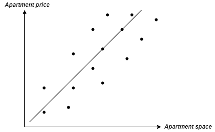Linear Regression Graph

The black regression line predicts where any of the points should be, based on the way the line was calculated. This means that the line represents what the value of the apartment should be, based on the total space of that apartment.

The distance between any point and the regression line represents how big the error is. The difference between how much an apartment costs (this is usually denoted as ŷ in practice)and how much it should cost is based on the market trend and the regression algorithm prediction (noted simply as y).

The question is, how is that linear regression line is calculated? How do you find how to predict y based on x?

The answer is, by taking each of the differences between the points on the graph and the line, squaring them, and adding them up. Then the algorithm moves the line until it finds the least squared sum of those points.

The formula for the least squared sum of the difference between predicted data and actual data is:


Least_Mean_Square_sum= min(Sum (ŷ-y)²)

This is calculated for each line, drawing many lines, and the line where the least mean square sum is the lowest is chosen.

Python Code

Here is a bit of code that will help you implement a simple linear regression in python3, from start to finish.

First, import the relevant libraries or install them if you haven’t and then import them. I highly recommend using Anaconda.

Also, before installing packages I recommend getting familiar with virtual environments in Anaconda. Be sure to read about this before starting coding, as it will save you a lot of headaches.


import numpy as np
import matplotlib.pyplot as plt
import pandas as pd
from sklearn.model_selection import train_test_split
from sklearn.linear_model import LinearRegression

Now we have to import the dataset.


dataset = pd.read_csv(‘Appartment_Price_Data.csv’)
X = dataset.iloc[:, :-1].values
y = dataset.iloc[:, -1].values

You then split the dataset into training and test set.


X_train, X_test, y_train, y_test = train_test_split(X, y, test_size = 1/3, random_state = 0)

Now we get to the fun part — training the linear regression model.


regressor = LinearRegression()
regressor.fit(X_train, y_train)

Now that we trained the model, it means that we can actually use the algorithm to predict the price of apartments based on space.


y_pred = regressor.predict(X_test)

If you wish to use matplotlib to also get some graphical representations you can add the following lines of code for the training dataset:


plt.scatter(X_train, y_train, color = ‘blue’)
plt.plot(X_train, regressor.predict(X_train), color = ‘black’)
plt.title(‘Apartment Price and Apartment Space (Training set)’)
plt.xlabel(‘Apartment Space’)
plt.ylabel(‘Apartment Price’)
plt.show()

And this code for the test dataset:


plt.scatter(X_test, y_test, color = ‘blue’)
plt.plot(X_train, regressor.predict(X_train), color = ‘black’)
plt.title(‘Apartment Price and Apartment Space (Test set)’)
plt.xlabel(‘Apartment Space’)
plt.ylabel(‘Apartment Price’)
plt.show()

Hope this will help you get some hands-on with this algorithm. You can use the code exactly as it is on any dataset that has 1 independent variable (X) and 1 dependent variable (y).
Conclusion

There are many other types of regression out there that I will cover in future articles. But for now, you should have at least some idea about what a regression is. Find other sources too, and code some regression algorithms, if you wish to truly master this “Hello World” of machine learning and data science method.

Stay focused and passionate and keep learning!